The MOSSE algorithm

Correlation filters

Filter-based object trackers locate an object by training a filter to model its appearance using multiple example images. The filter scans (or correlates) over a search window to determine the object's position in the image.

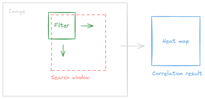
This can get quite slow however, especially for real-time applications.

The fast fourier transform trick

One strategy that has been quite successful to speed up things is the use of the Fourier transform. This trick involes computing the correlation in the frequency domain instead of the spatial domain. Instead of sliding the filter across each position of the image, we can get our correlation result in one go by multiplying it all in the frequency domain (convolution theorem).

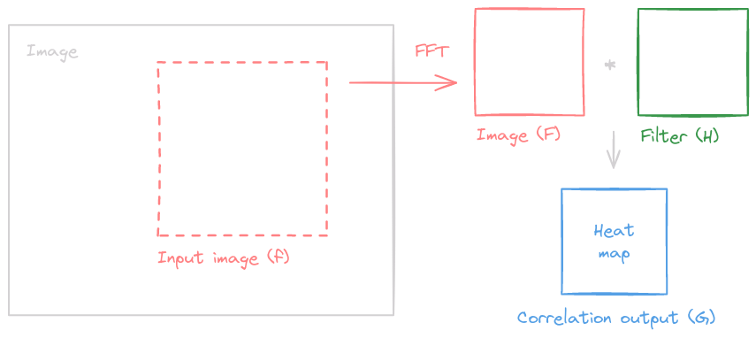
Definitively dark magic!

Let's build it

The preprocessing step

At each step of the algorithm the images are preprocessed to improve the correlation results. In MOSSE, the authors use the preprocessing steps described in Average of Synthetic Exact Filters.

1. Log transformation: reduces the effect of shadows and intense lightning.

   def log_transform(image: np.ndarray) -> np.ndarray:
       return np.log(image + 1)

2. Normalization to zero mean and squared sum of one: creates more consistent values.

   def normalize(image: np.ndarray) -> np.ndarray:
       return (image - image.mean()) / (image.std() + 1e-5)

3. Use of a cosine window: reduces the frequencies at the edges of the image

   def hanning_window(image: np.ndarray) -> np.ndarray:
       height, width = image.shape
       mask_col, mask_row = np.meshgrid(np.hanning(width), np.hanning(height))
       window = mask_col * mask_row
       return image * window

The initialization step

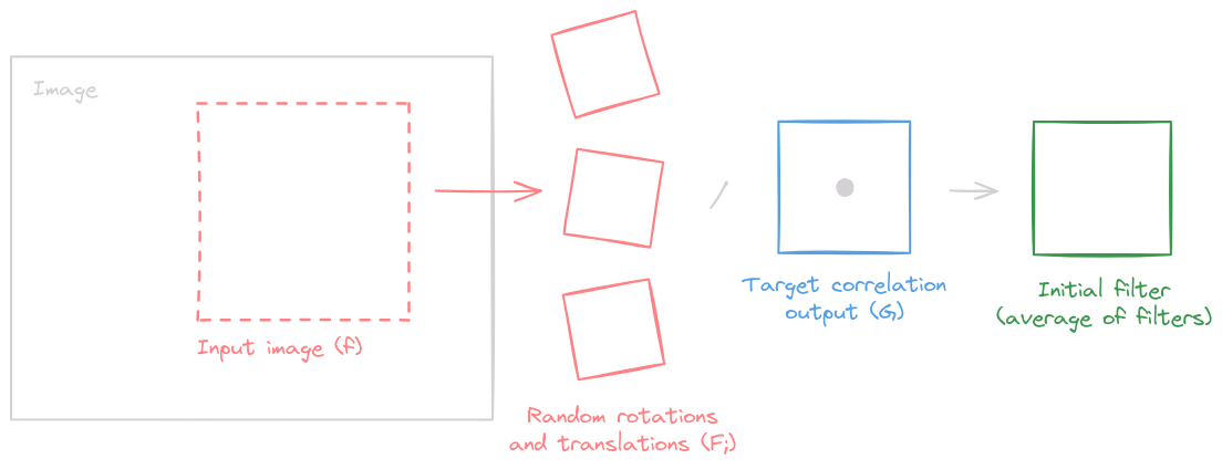
The first step is to initialize the filter. The relationship between the filter, the template and the image in the Fourier domain is defined as: $$ G = F \odot H^{*} \hspace{1cm} \text{and} \hspace{1cm} H^{*} = \dfrac{G}{F} $$

However, as this filter overfits the first frame, it can fail to generalize to the next frames. To overcome this, MOSSE applies multiple random transformations and averages the filters to make it more robust.

The update step

When updating the filter with new frames, MOSSE finds a filter that optimzes the following objective function: $$ \min_{H^{*}} \sum_{i} \left| F_{i} \odot H^{*} - G_{i} \right|^{2} $$ This optimization problem can be solved using the following equation: $$ H^{*} = \dfrac{\sum_{i} F_{i} \odot G_{i}^{*}}{\sum_{i} F_{i} \odot F_{i}^{*}} $$ MOSSE uses a running average with a learning rate η to update the filter: $$ H^{*} = \dfrac{A_{i}}{B_{i}} $$ $$ A_{i} = \eta G_{i} \odot F_{i}^{*} + (1 - \eta) A_{i - 1} \hspace{1cm} and \hspace{1cm} B_i{i} = \eta F_{i} \odot F_{i}^{*} + (1 - \eta) B_{i -1} $$ All of the details are available in the original paper.